Predicting the Success of Bank Telemarketing
Introduction
In this case study, we are going to explore the processes involved in a typical data mining task. When building a predictive model, there are some common problems you are likely to meet in your data - problems such as missing values, imbalanced classes, un-informative attributes and so on. Here we shall look at some proven techniques for dealing with such problems and many other important guidelines.
We shall make an attempt to understand some functions that can make your life easier when working on projects in r
I hope to provide a strong foundation for solving more challenging and complicated problems with data. If you are new to data science and are interested in learning, then I’ll encourage you to download the data in the link provided below and follow each step religiously.
Problem Discription And Objectives
Financial Institutions such as Banks, Savings and Loans cooperation often provide cash investments services for their customers, one of such investment service is the term deposits. A term deposit is simply a cash investment held at a financial institution over a fixed amount of time. When a term deposit is purchased from a bank, the customer understands that the money can only be withdrawn after the term has ended or by giving a predetermined number of days notice.
Now, these financial institutions need lot of customers to deposit money with them, the reason is because they use these deposits to do business and earn profits for their organization. When a customer deposits money, the bank would lend it out and make interest on it.
A financial institution is launching a new marketing campaign and In order to minimize cost and optimize strategy, managment has decided to employ data scientist to leverage on their past data and target only the customers who would subscribe to their offer
Looking at historical data on customers who have been targeted with similar products, we shall build a model to estimate how likely a customer would respond to this new offer.
These case study walks us through an intelligent way of building a good model that would classify your customers appropriately
Data Description
The data is related with direct marketing campaigns of a Portuguese banking institution. The marketing campaigns were based on phone calls. Often, more than one contact to the same client was required, in order to access if the product (bank term deposit) would be (‘yes’) or not (‘no’) subscribed.
The data can be downloaded from the UCI Machine Learning Repostitory. The classification goal is to predict if the client will subscribe a term deposit (variable y).
Attribute Information:
- Age
- Job - type of job
- marital - marital status
- Education - Shows the level of education of each customer
- Default - Whether a customer has credit in default
- Housing - Does the customer have a housing loan?
- Loan - Does the customer have a personal loan?
- Contact - The contact communication type
- Month - Last contact month of year
- day_of_week - Last contact day of Week
- Duration - Last contact duration in seconds
- Campaign - Number of contact performed for the client during the campaign
- pdays: number of days that passed by after the client was last contacted from a previous campaign
- previous: number of contacts performed before this campaign and for this client
- poutcome: outcome of the previous marketing campaign
- emp.var.rate: employment variation rate - quarterly indicator
- cons.price.idx: consumer price index - monthly indicator
- cons.conf.idx: consumer confidence index - monthly indicator
- euribor3m: euribor 3 month rate - daily indicator
- nr.employed: number of employees - quarterly indicator
The Output variable (Desired Target)
- y - has the client subscribed a term deposit? (binary: ‘yes’,‘no’)
Reading the Data into R
The data can be read directly from your browser through the link provided above, or you can download the data into your computer and follow the steps below to get it into R.
readr comes with several functions for reading flat file data into R The advantage readr has over it’s equivalent base functions is it’s speed - readr is 10x faster than base r
we use read_csv2 function to read our semicolon delimited file into R:
# contains readr
library(tidyverse)
library(knitr)

# Load Data
raw_data <- read_csv2("/home/dreamadmin/Desktop/bank/bank-additional-full.csv")
#raw_data <- bank_additional_full


kable(head(raw_data))| age | job | marital | education | default | housing | loan | contact | month | day_of_week | duration | campaign | pdays | previous | poutcome | emp.var.rate | cons.price.idx | cons.conf.idx | euribor3m | nr.employed | y |
|---|---|---|---|---|---|---|---|---|---|---|---|---|---|---|---|---|---|---|---|---|
| 56 | housemaid | married | basic.4y | no | no | no | telephone | may | mon | 261 | 1 | 999 | 0 | nonexistent | 11 | 93994 | -364 | 4857 | 5191 | no |
| 57 | services | married | high.school | unknown | no | no | telephone | may | mon | 149 | 1 | 999 | 0 | nonexistent | 11 | 93994 | -364 | 4857 | 5191 | no |
| 37 | services | married | high.school | no | yes | no | telephone | may | mon | 226 | 1 | 999 | 0 | nonexistent | 11 | 93994 | -364 | 4857 | 5191 | no |
| 40 | admin. | married | basic.6y | no | no | no | telephone | may | mon | 151 | 1 | 999 | 0 | nonexistent | 11 | 93994 | -364 | 4857 | 5191 | no |
| 56 | services | married | high.school | no | no | yes | telephone | may | mon | 307 | 1 | 999 | 0 | nonexistent | 11 | 93994 | -364 | 4857 | 5191 | no |
| 45 | services | married | basic.9y | unknown | no | no | telephone | may | mon | 198 | 1 | 999 | 0 | nonexistent | 11 | 93994 | -364 | 4857 | 5191 | no |
Summarizing the Data
Once you have imported your data, the next step I’ll recommend is to calculate a set of summary statistics on it. Summarizing your data is very useful because it kind of reduces your bulk data into something you can understand and interpret
What to look out for when summarizing your data includes: mean, median inter-quatile range, count of values and so on. The dim() function also displays the dimension of the dataset, in this dataset, we have 41188 instances and 21 attributes. Below are some basic functions in R, that provide you with a range of descriptive statistics at once.
# glimpse(raw_data)

summary(raw_data)

dim(raw_data)
Create two Data Frames from your Data
We shall divide our dataset into two - one for numerical variables and the other for categorical variables. This is a good option to consider when you are about exploring your data. You can easily identify problems that are peculiar to each type of vectors and iterate over each vector conveniently when solving those problems
We used the map functions from the purr package - this functions are very useful for manipulating vectors. You can read more on the purr package by clicking here
num <- map_lgl(raw_data, is.numeric)

num_var <- raw_data[, num]

char_var <- raw_data[, !num]

# Add the target variable to the numeric variables
num_var <- num_var %>%
        mutate(y = char_var$y)
Visualize the Data
Data Visualization helps you quickly spot surprises in your data. A good visualization makes complex data more understandable.
An Histogram is typically used to visualize the distribution of a numeric variable whereas the bar graphs are used for the categorical variables. In both bar charts and histograms, tall bars show the common values of a variable, and shorter bars show less-common values. You should always explore a variety of binwidths when working with histograms, as different binwidths can reveal different patterns.
ggplot(num_var, aes(x = age)) +
        geom_histogram(fill = "skyblue", color = "black") +
  theme_bw()
## `stat_bin()` using `bins = 30`. Pick better value with `binwidth`.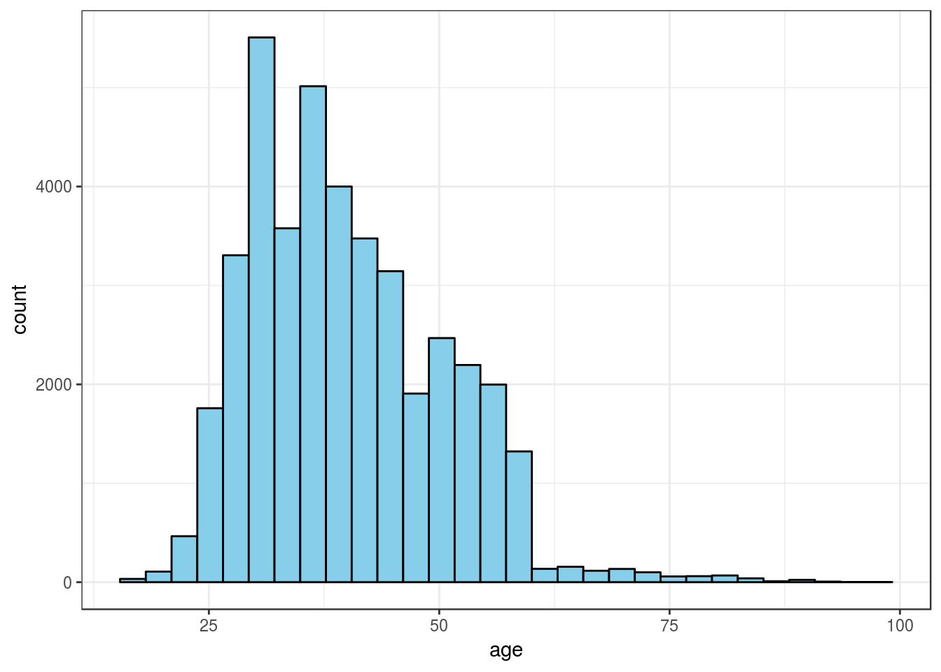
To avoid copying and pasting the code. I have written a function for plotting the histograms on each numeric variable
plot_hist <- function(x, bins = 40){
        ggplot(num_var, aes(x = x)) +
                geom_histogram(fill = "white", color = "black",
                               bins = bins)

plot_hist(num_var$duration, bins = 100)

}
Important note: this attribute (duration) highly affects the output target (e.g., if duration=0 then y=‘no’). Yet, the duration is not known before a call is performed, also the end of the call y is obviously known. Thus, this input should only be included for benchmark purposes and should be discarded if the intention is to have a realistic predictive model.
ggplot(num_var, aes(x = y, y = duration)) +
        geom_boxplot() +
  theme_bw()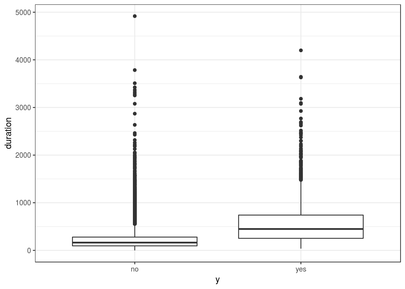
ggplot(char_var, aes(job, fill = y)) +
        geom_bar(position = "dodge", color = "black") +
        scale_fill_brewer(palette = "Pastel1") +
        theme(axis.text.x = element_text(angle = 45, hjust = 1)) +
  theme_bw()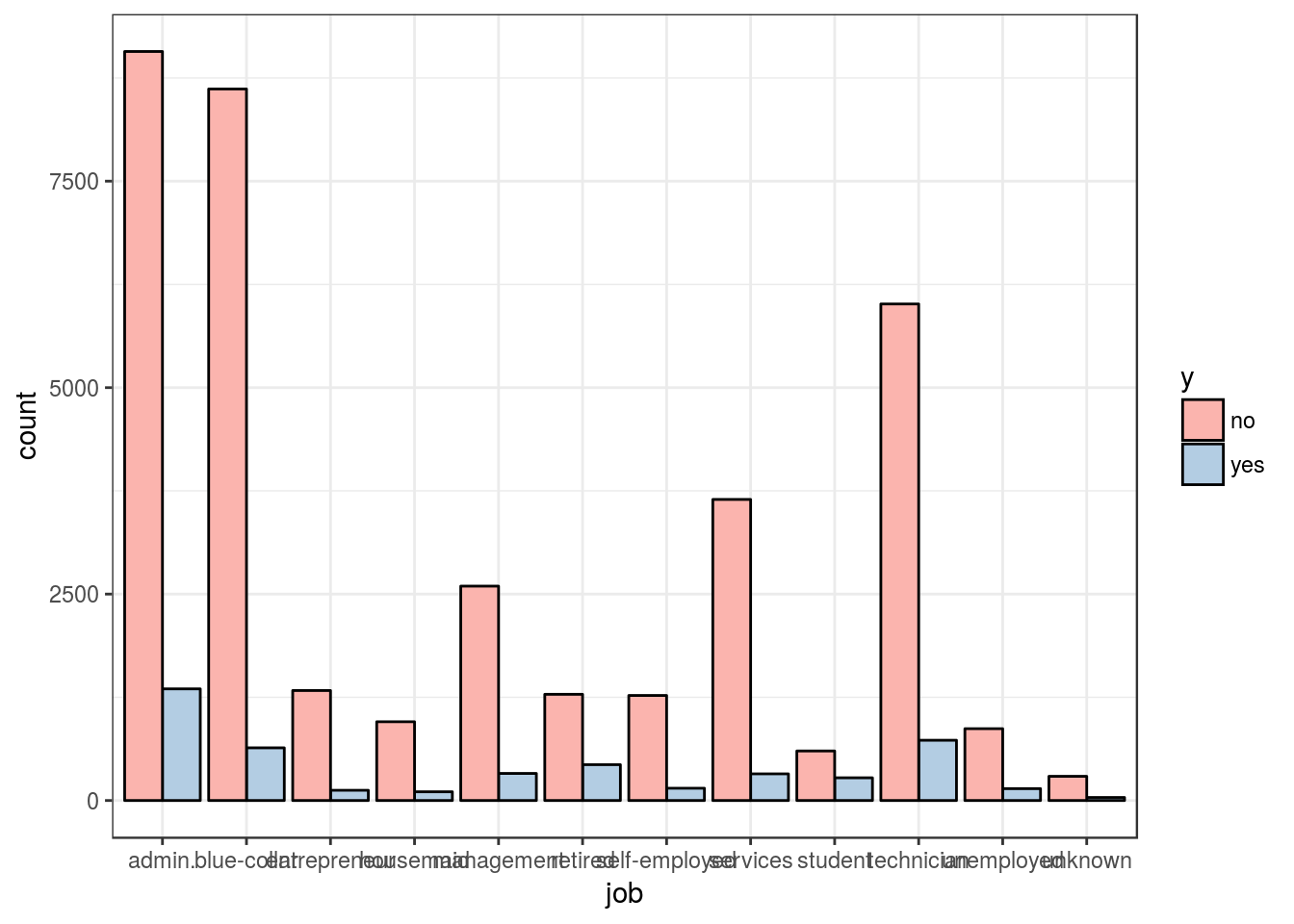
I’ll write a function to plot the categorical variables. Functions prevents unecessary duplication in your codes.
plot_char <- function(x){
        ggplot(char_var, aes(x, fill = y)) +
                geom_bar(position = "dodge", color = "black") +
                scale_fill_brewer(palette = "Pastel1") +
                        theme(axis.text.x = element_text(angle = 45, hjust = 1))

}


plot_char(char_var$education)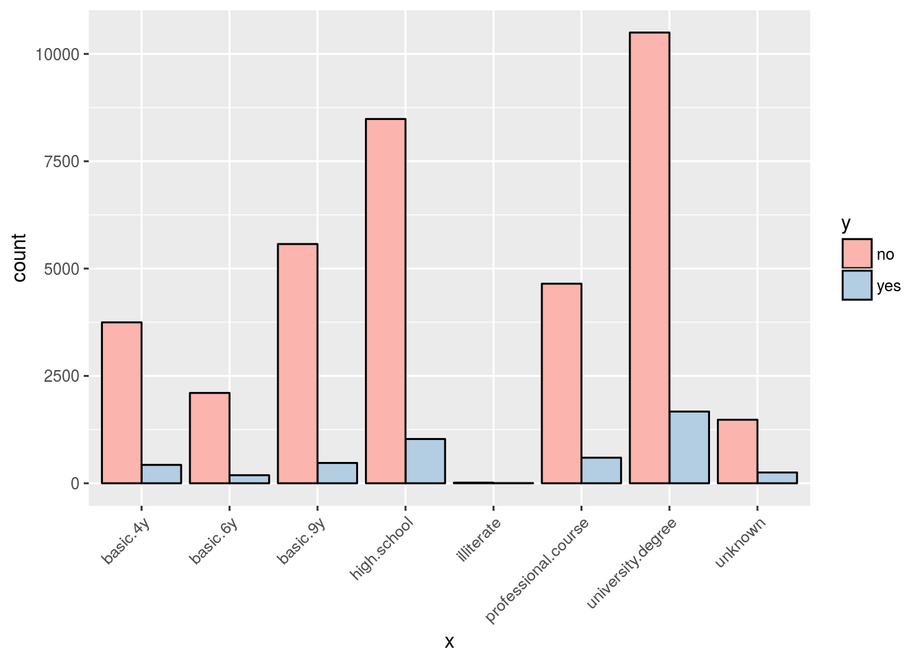
Data Transformation:
A very important aspect of data science is getting the data in the right form for analysis. Very few data can be considered perfect. We look at some ways to get our data into the right format in order to achieve optimal results
Dealing with Missing Values
The presence of missing data is a common problem you see on real datasets. When dealing with missing values, we should first and foremost find out if the pattern of the missing data is related to the outcome. Missing values may be concentrated in a subset of predictors or could occur randomly accross all the predictors. In many cases it is ideal to remove a predictor if the proportion of missing values in it is very high.
i found that 33425 values were missing from the nr.employed variable. That represent 81.1522774 percentage of missing values. Hence i removed this variable from subsequent modeling activities. We use a function from the dplyr package - select() - which allows you to rapidly zoom in on a useful subset of columns
map_dbl(num_var, function(x)sum(is.na(x)))## age duration campaign pdays previous
## 0 0 0 0 0
## emp.var.rate cons.price.idx cons.conf.idx euribor3m nr.employed
## 0 0 0 0 33425
## y
## 0num_var <- select(num_var, -nr.employed)Condence low frequency character values
From our exploratory graphs, we observe that many of the attributes (categorical variables), have levels with very low frequenies. Since the purpose of the model is to find patterns in the data that can generalize to an unseen data - levels with low frequency are better combined together. This is because those low frequency levels may not be present in the test data.
I wrote a function below to combine levels having a frequency less that 2% of the values in the data. The map funtion below loops over the character variables and generate result that have low frequency levels combined
combine_levels <- function(x, threshold = 0.02) {
  lowLevels <- names(which(prop.table(table(x)) < 0.02))
  x[x %in% lowLevels] <- "other"
  x
}

char_var <- map_df(char_var, combine_levels)


# make categorical variable factors
conv_to_factors <- function(x){
        as.factor(x)
}


fac_var <- map_df(char_var, conv_to_factors)


# Convert some low variance numeric variables to categorical
# and condense levels with values less than 5%

num_var$pdays <- ifelse(num_var$pdays == 999, "not_contacted", "contacted")
num_var$pdays <- combine_levels(num_var$pdays)
num_var$pdays <- conv_to_factors(num_var$pdays)

num_var$previous <- as.character(num_var$previous)
num_var$previous <- combine_levels(num_var$previous)
num_var$previous <- conv_to_factors(num_var$previous)

num_var$campaign <- as.character(num_var$campaign)
num_var$campaign <- combine_levels(num_var$campaign)
num_var$campaign <- conv_to_factors(num_var$campaign)

num_var <- select(num_var, -duration, -y)
Resolving collinearity
When predictors are correlated with other predictors in your data, then there is an issue of collinearity. Using highly correlated predictors in some modeling techniques can result in highly unstable models and produce poor predictive performance
There is a function in the caret package that searches through a correlation matrix and points out columns to remove in order to reduce pair-wise correlations.
library(caret)
library(corrplot)

bank_data <- cbind(num_var, fac_var)

corMatrix <- cor(bank_data[, c(1, 5:8)])

# correlation plot
corrplot(corMatrix, order = "hclust", tl.cex = .65)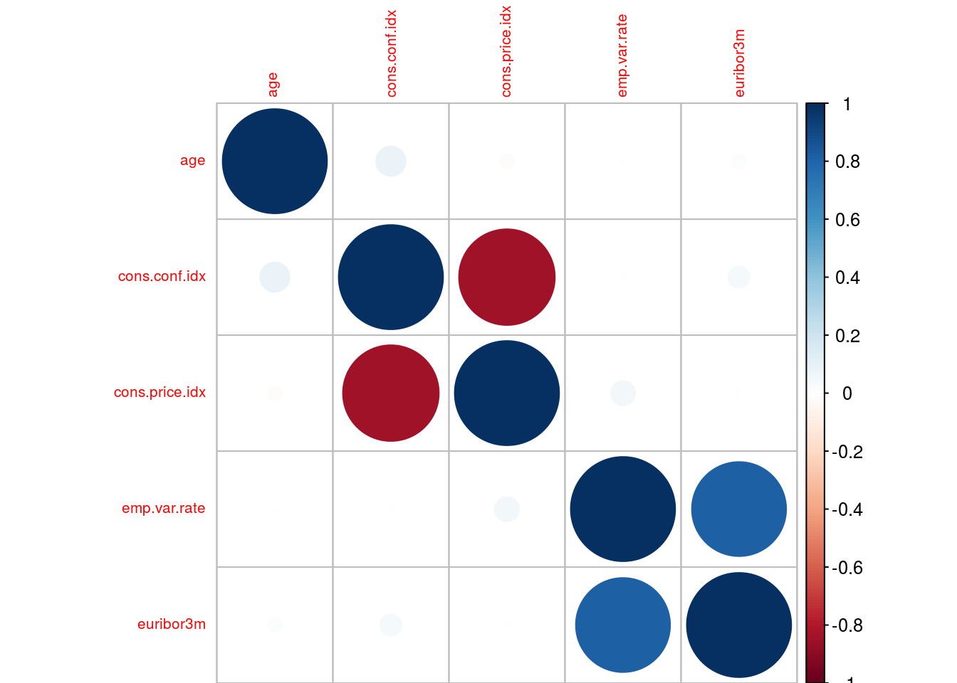
highCor <- findCorrelation(corMatrix, cutoff = .75)
bank_data <- bank_data[, -c(7:8)]
Obtaining Prediction Models
The main goal of this case study is to predict whether or not a client would subscribe a term deposit from a banking institution. We’ll simply use our data and some machine learning techniques to identify the customers who purchased the term deposit.
In general, machine learning is about learning to do better in the future based on experience from the past.
The focus is to provide high-level predictions that guide better decisions without human interventions.
Partition your data into training and test set.
One of the first decisions to make when modeling is to decide which samples will be used to evaluate your model’s performance. The training data set is the general term for the samples used to create the model, while the test set is what is used to measure performance
With many data science applications - like the one we are working on right now, the proportion of the classes are substantially different therefore when splitting your data into a training and a test set, take that into account. caret provides a function that splits the data using stratified random sampling, which takes into account the difference in classes
outcome <- bank_data$y

predictors <- select(bank_data, -y)


# partition data:

idx <- createDataPartition(outcome, p = 2/3,
                           list = FALSE)

predictors_train <- predictors[idx, ]
outcome_train <- outcome[idx]

predictors_test <- predictors[-idx, ]
outcome_test <- outcome[-idx]
Resolving Class Imbalance
An imbalance occurs when one or more classes have very low proportion in the training data as compared to the other classes - this phenomenon can have a significant impact on the effectiveness of the model. For instance, in our data, the outcome - whether or not the customer purchased a term deposit, is highly unbalanced with only 11% of customers having purchased a term deposit. 89, 11.
There are two general approaches that can be used to alleviate the effects of imbalance during model training. They are:
Up-sampling: this is a technique that imputes additional data points to improve balance across classes.
Down-sampling: reduces the number of samples to improve the balance accross classes
The synthetic minority over-sampling technique (SMOTE) is a data sampling procedure that uses both up-sampling and down-sampling, depending on the class. In this case study we applied SMOTE to the random forest model for the bank telemarketing data. A function for SMOTE can be found in the DMwR package.
library(DMwR)
set.seed(10)
smooth_data <- SMOTE(y ~., data = bank_data)


outcome_train <- smooth_data$y
predictors_train <- select(smooth_data, -y)


round(prop.table(table(outcome_train))*100)
## outcome_train
## no yes
## 57 43We see the improvments in the proportion of class frequency after applying the SMOTE
Almost all predictive modeling techniques have tuning parameters that enable the model to flex to find the structure in the data. We use resampling techniques, such as cross-validation, to choose the best parameters for optimal performance. Also, train can use standard resampling methods for estimating performance
ctrl <- trainControl(method = "cv",
                     summaryFunction = twoClassSummary,
                     classProbs = TRUE)
We shall build our model using random forest. You can read about random forest from Wikipedia. The train function contains wrappers for tuning the random forest models by specifying either method = “rf”. Optimizing the mtry parameter may result in a slight increase in performance.
rfFit <- train(x = predictors_train,
               y = outcome_train,
               method = "rf",
               ntree = 500,
               importance = TRUE,
               metric = "ROC",
               trControl = ctrl)
Measure Models performance:
We shall use the ROC curve to qualify the performance of our model. A definition from wikipedia defines ROC curve thus:
In statistics, a receiver operating characteristic (ROC), or ROC curve, is a graphical plot that illustrates the performance of a binary classifier system as its discrimination threshold is varied
A perfect model that completely separates the two classes would have 100% sensitivity and specificity.
Sensitivity is the accuracy rate for only the positive class, in this case customers who purchased the term deposit while specificity is the accuracy rate for the negative class - customers who did not purchase a term deposit
One advantage of using ROC curves to characterize models is that, since it is a function of sensitivity and specificity, the curve is insensitive to disparities in the class proportions
# Obtain test Result.
testResult <- predict(rfFit, predictors_test)

confusionMatrix(outcome_test, testResult,
                positive = "yes")
## Confusion Matrix and Statistics
##
## Reference
## Prediction no yes
## no 11552 630
## yes 47 1499
##
## Accuracy : 0.9507
## 95% CI : (0.9469, 0.9542)
## No Information Rate : 0.8449
## P-Value [Acc > NIR] : < 2.2e-16
##
## Kappa : 0.7881
## Mcnemar's Test P-Value : < 2.2e-16
##
## Sensitivity : 0.7041
## Specificity : 0.9959
## Pos Pred Value : 0.9696
## Neg Pred Value : 0.9483
## Prevalence : 0.1551
## Detection Rate : 0.1092
## Detection Prevalence : 0.1126
## Balanced Accuracy : 0.8500
##
## 'Positive' Class : yes
## Our random forest model correctly predicted 70% of customers who purchased the term deposit and about 99.7% of customers who did not purchase the term deposit.
View the important variables:
When training a tree, you can compute how much each feature decreases the weighted impurity in the tree. For a random forest, the impurity decrease from each feature can be averaged and the features are ranked according to this measure
varImpPlot(rfFit$finalModel,type=2, main = "Dotchart of Variable Importance")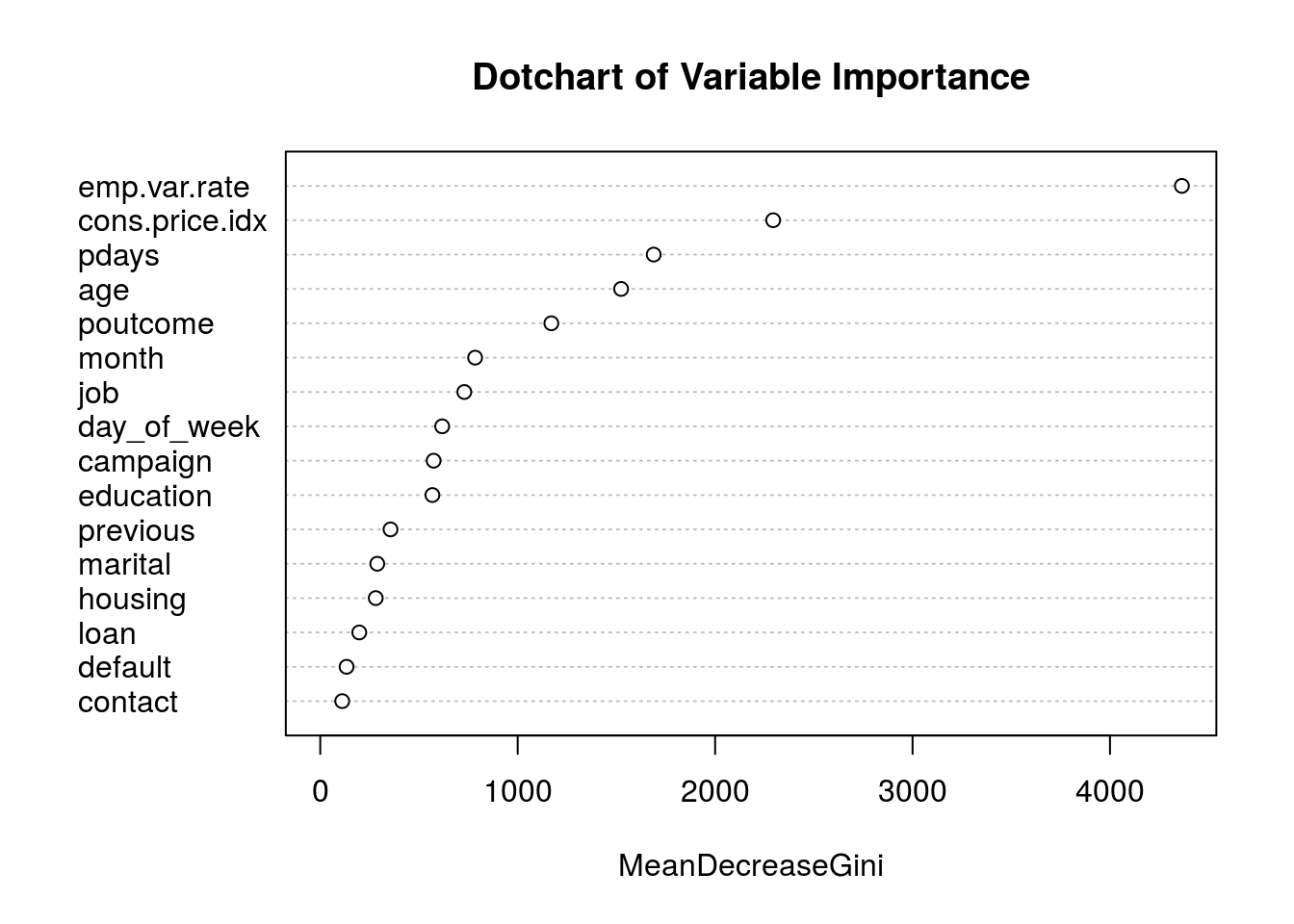
We may decide to remove the less important features from the set of predictors, re-build the model with the reduced features and check for improvements in performance.
Summary
We were provided with an historical data of customers targeted during a marketing campaign from a banking instution and our goal was to build a classification model that would accurately predict which customers would subscribe a term deposit in a new marketing campaign
We walked through the model building process and highlighted some peculiarities with the data. A unique feature of the data was that the classes were imbalanced, we studied a technique for solving the problem. We also learnt some functions in the caret package for building our model. Our accuracy on the event of interest was good and we pointed out ways to improve the model
let me know your thoughts in the section below:
